Quality control pipeline
On this page we detail the quality control (QC) pipeline for the UK Biobank exomes before starting our analyses. Further plots and the underlying code can be found on the SAIGE gene munging github repository.
For our QC pipeline, we first perform a collection of careful QC steps. The
initial step in this process is to read in the .vcf files,
split multiallelics and realign indels, and calculate a collection of
sample-level statistics.
Initial sample filtering
- Filter out samples based on MAD thresholds.
Initial genotype filtering
Our next step (after conversion of the joint called .vcf
file to a hail matrix table) is to remove genotypes based on the
following collection of criteria:
- Remove if at least one of the following is true:
- Genotype quality \(<\) 20
- Depth \(<\) 10
- If heterozygous and a SNP:
- P-value from 1-sided binomial test of alt allele read depth relative to ref+alt read depth \(<\) 10-3
- If heterozygous and an indel:
- Alternative allele depth divided by total depth \(<\) 0.3
Initial variant filtering
Remove variants that either:
- Are invariant after the initial GT filter
- Fall in a low complexity region
- Fall outside padded target intervals (50bp padding)
- Have GATK ExcessHet > 54.69
Following this initial curation we perform a series of further QC steps detailed in this repository.
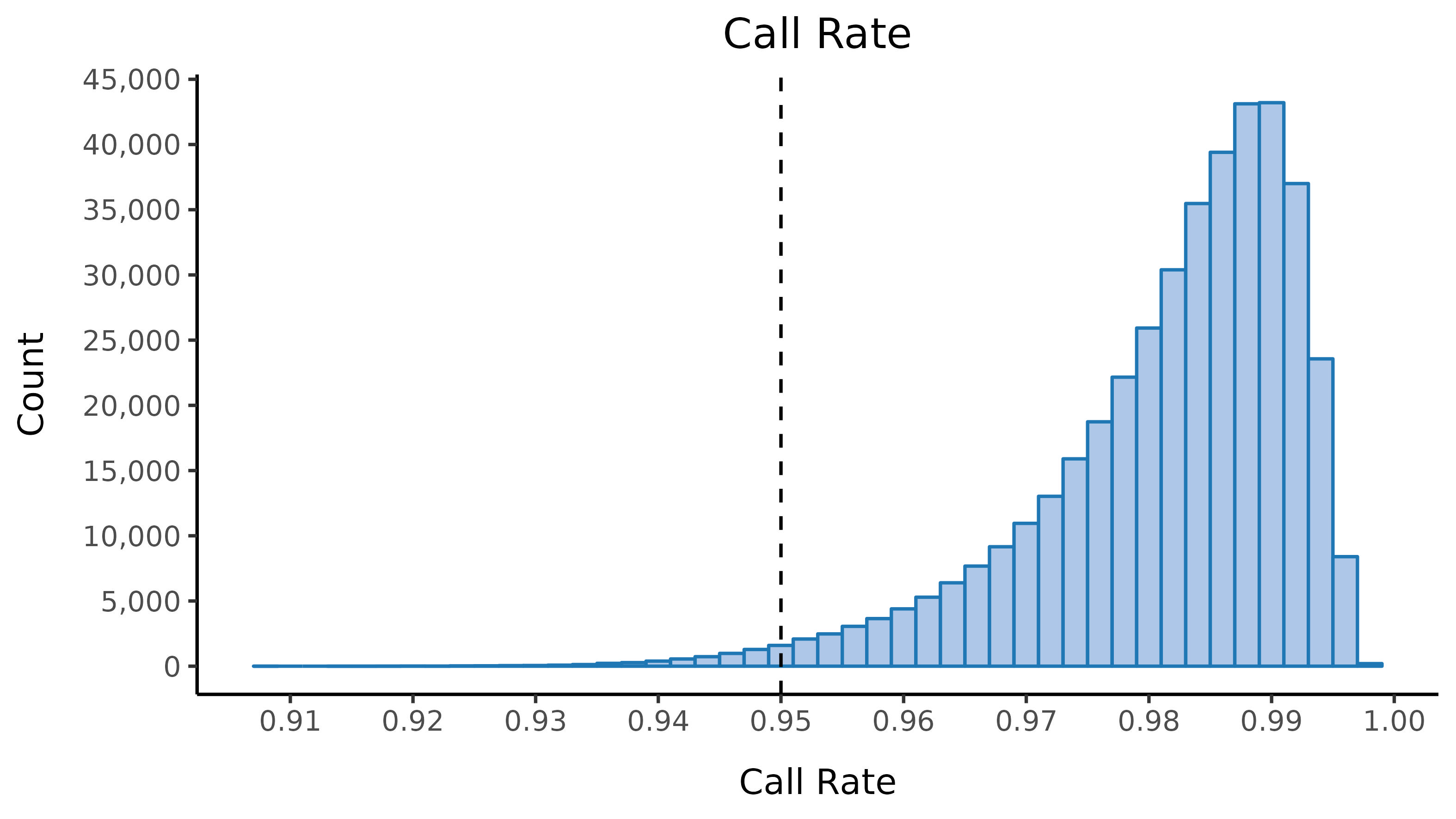
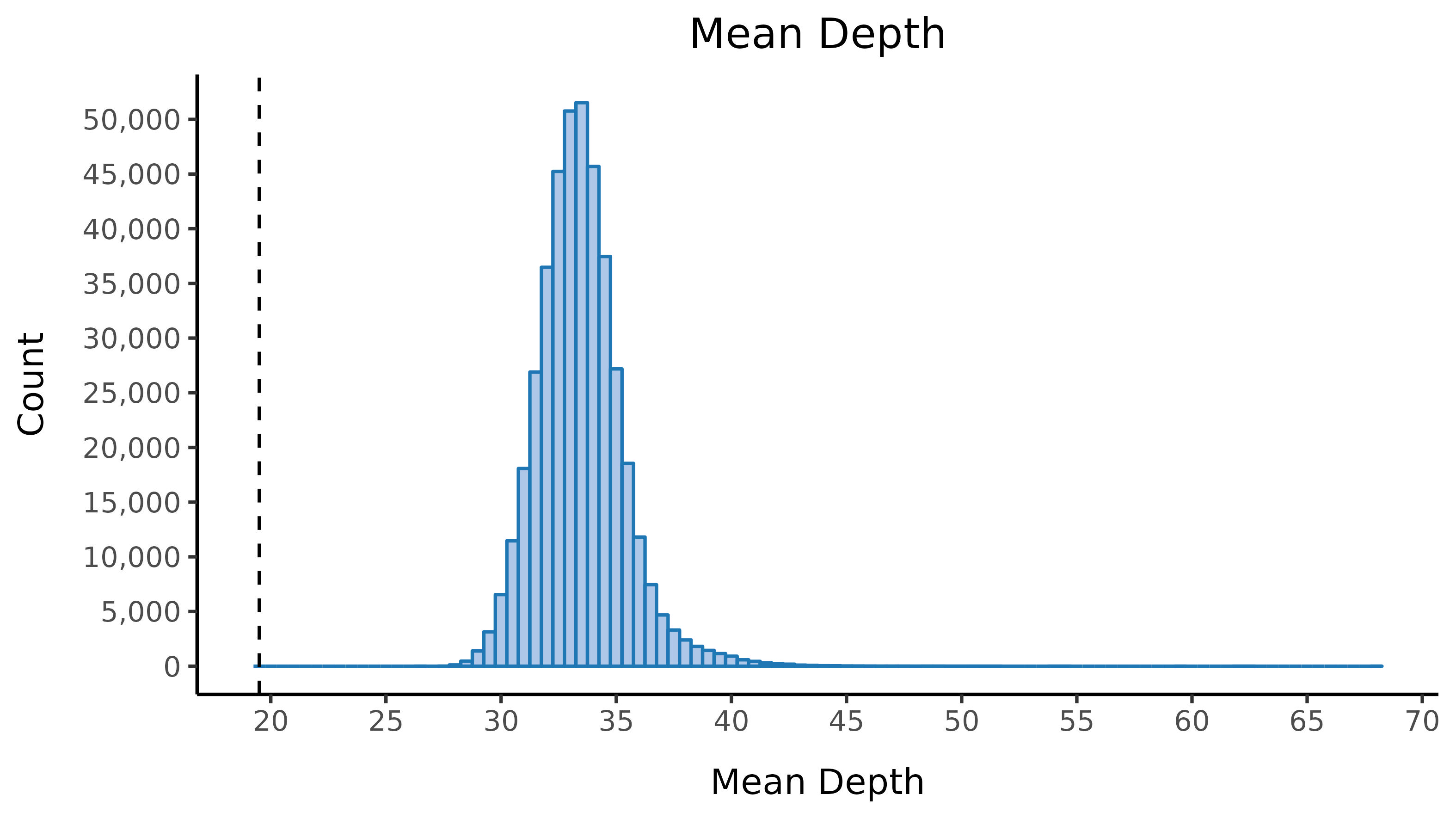
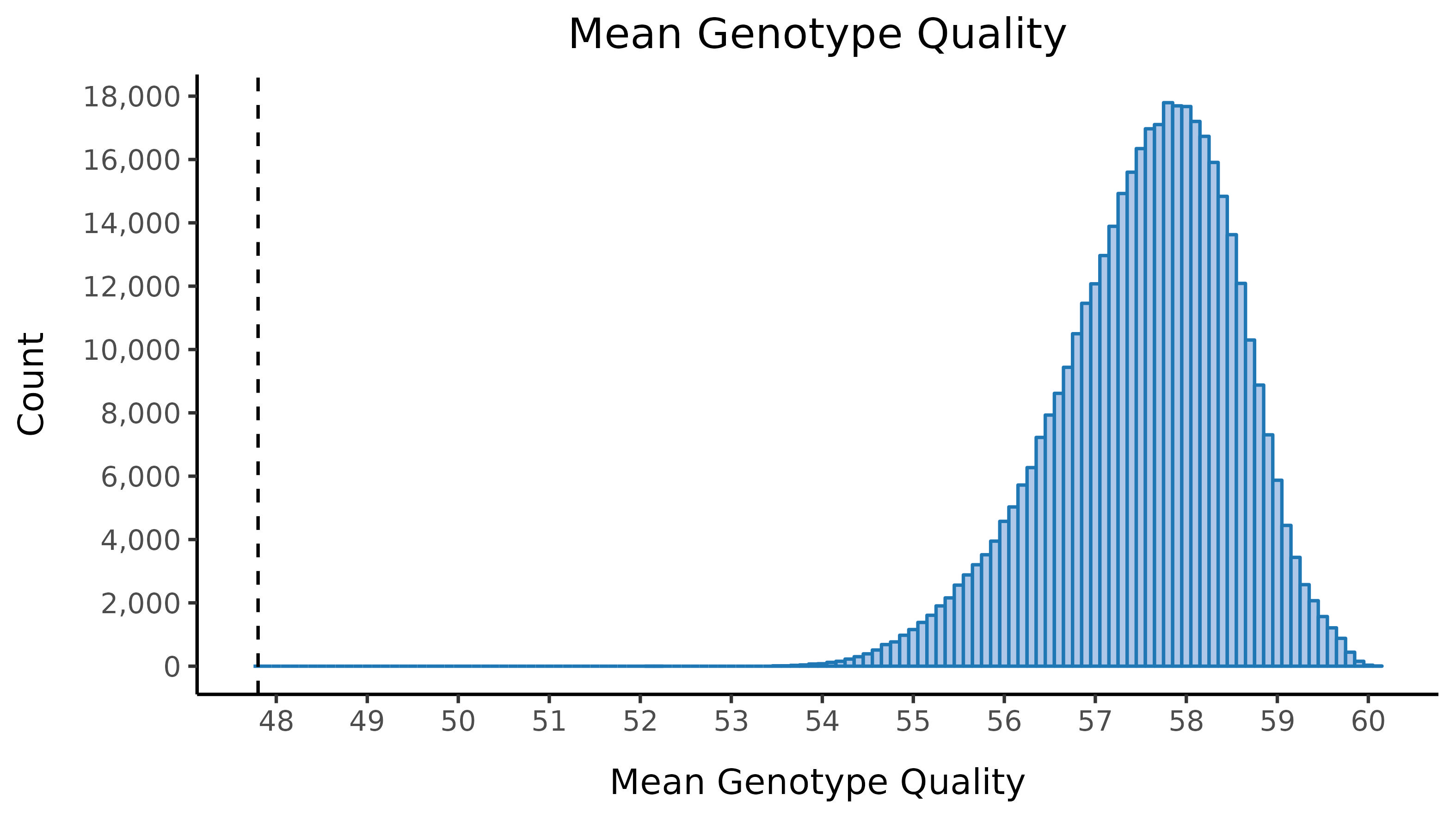
We run the sample_qc function in hail and remove samples according to the following:
- Sample call rate \(<\) 0.95
- Mean depth \(<\) 19.5
- Mean genotype quality \(<\) 47.8
Thresholds used were based on plotting the distributions of these metrics. Here we show boxplots with overlaid scatterplots of the above metrics, split by UKBB centre, and coloured by sequencing batch. The threshold for exclusion is shown as a dashed line.
| Filter | Samples | % |
|---|---|---|
| Samples after initial filter | 418,045 | 100.0 |
| Sample call rate | 5,537 | 1.3 |
| Mean DP | 0 | 0.0 |
| Mean GQ | 0 | 0.0 |
| Samples after sample QC filters | 412,508 | 98.7 |
Following this step, we export genotyped variants on the X chromosome
(allele frequency between 0.05 to 0.95 with high call rate (> 0.98))
to plink format and prune to pseudo-independent SNPs using
--indep 50 5 2. This pruned set of SNPs feeds into the sex
imputation step.
PCA to assign broad scale ancestry based on 1000 genomes labels
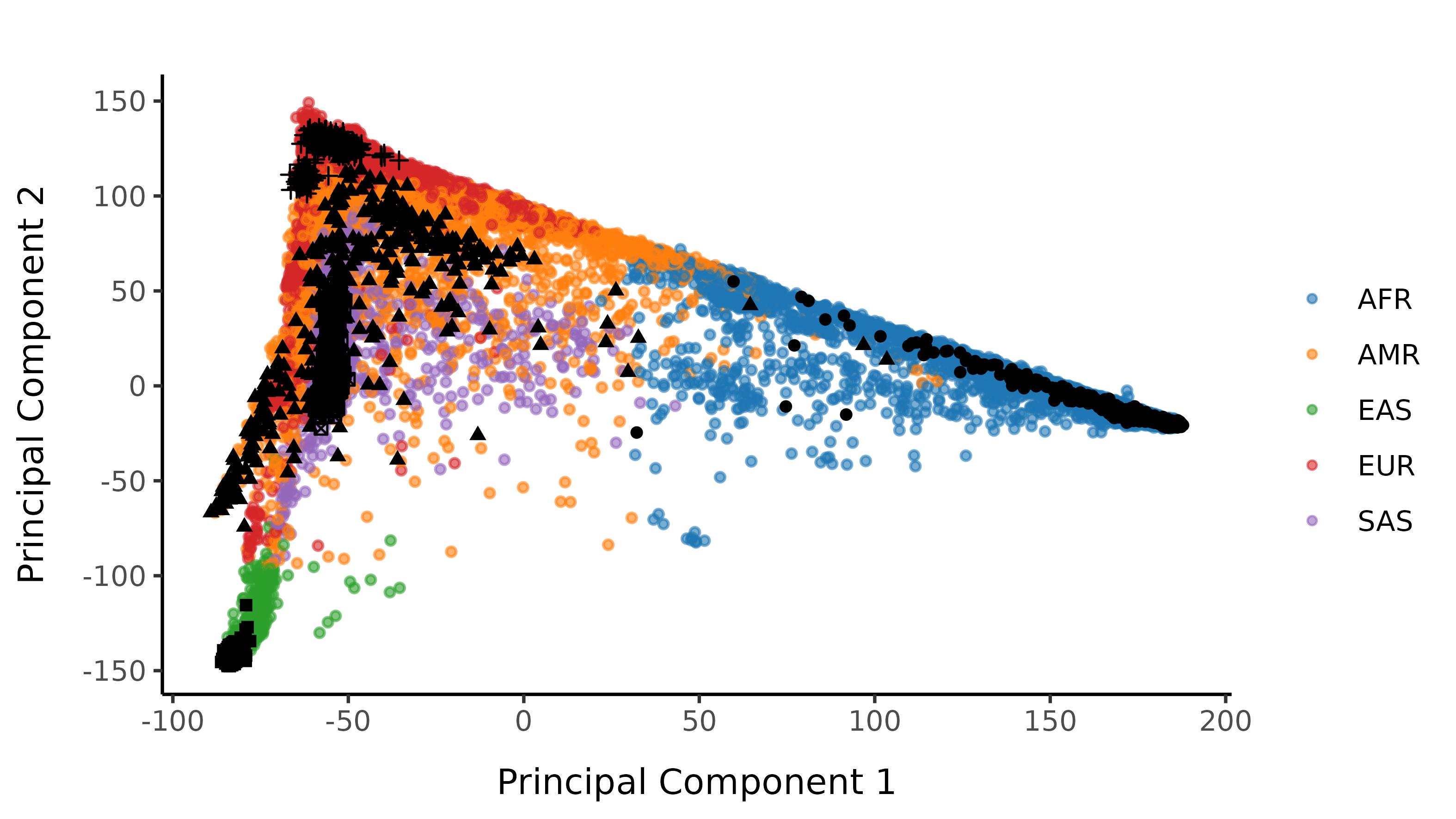
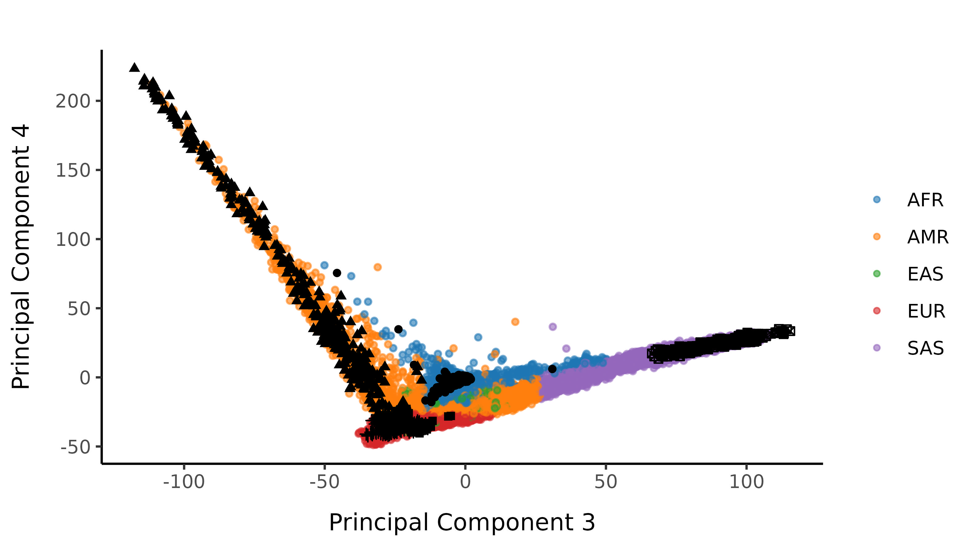
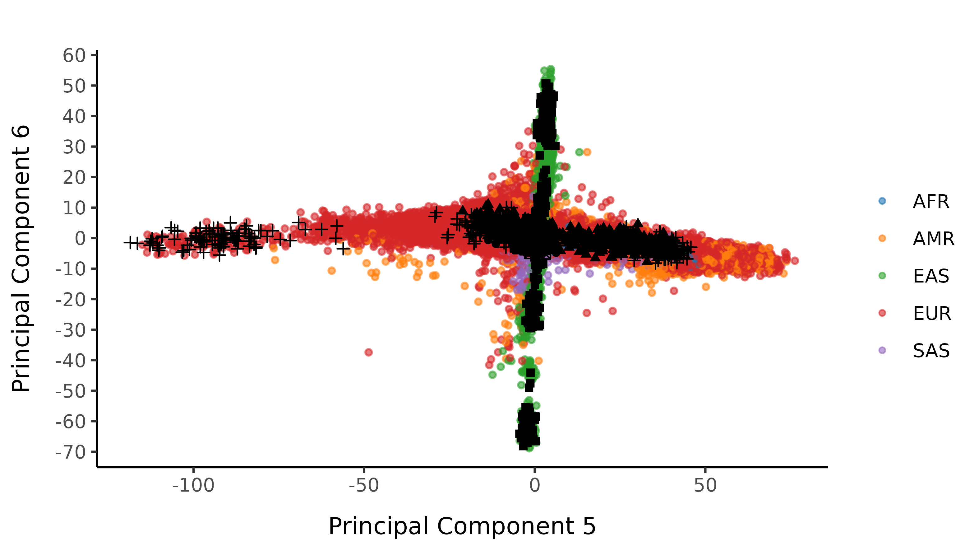
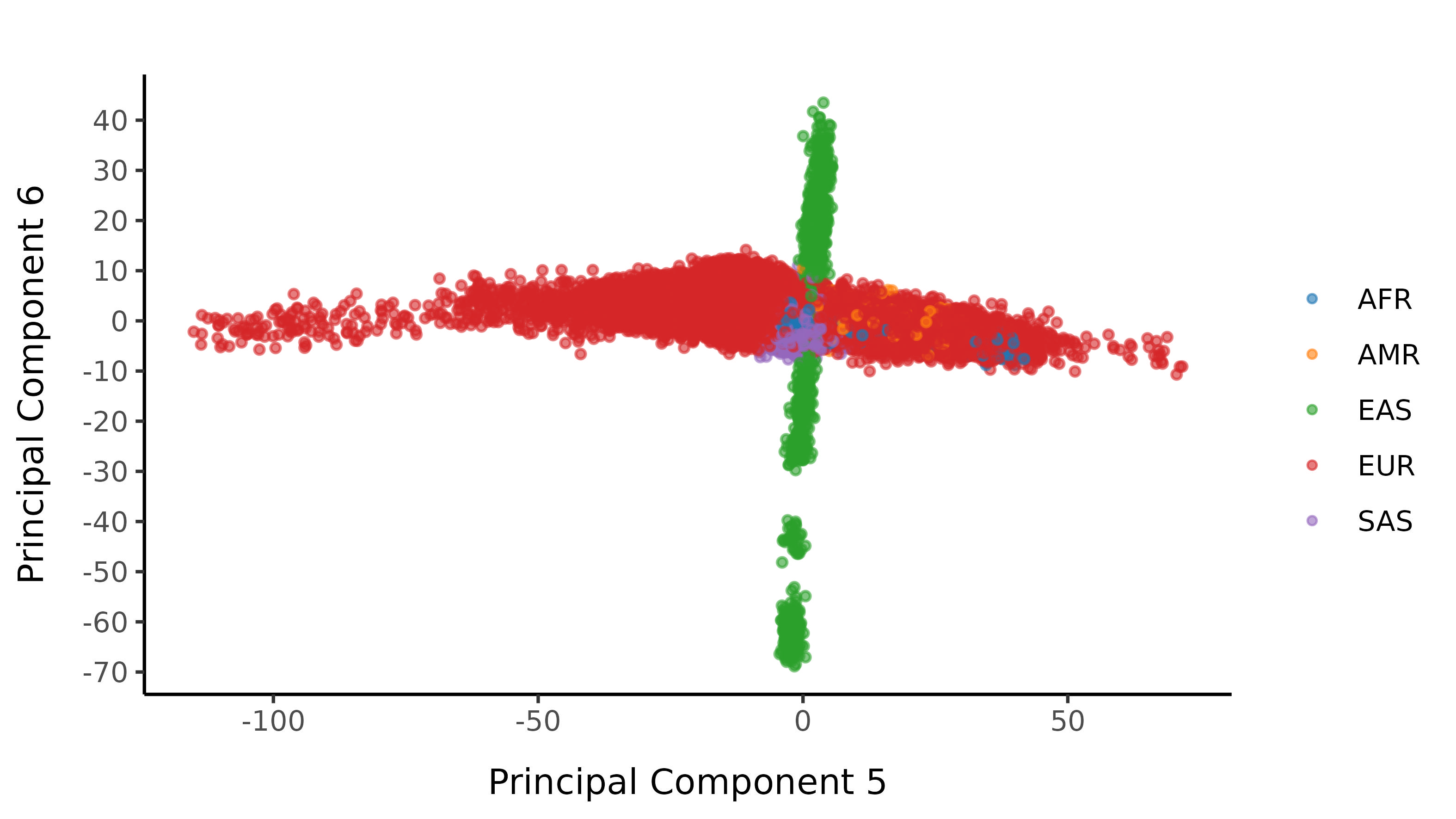
We next perform a number of principal component analysis (PCA) steps to label with broad scale ancestry.
We first run PCA on the 1000 genomes samples (minus the small subset of related individuals within 1000 genomes). We then project in the UK Biobank samples, ensuring that we correctly account for shrinkage bias in the projection.
We then train a classifier to assign 1000G population labellings. To do this, we train a random forest on the super populations labels of 1000 genomes and predict the super population for each of the UK Biobank samples. We denote strictly defined European subset as those with probability \(>\) 0.99 of being European according to the classifier. UK Biobank samples are coloured by their assignment or unsure if none of the classifier probabilities exceeded 0.99 in the following plots.
Here is the loose classifier, with no probability restriction on classification:
Following the Strict Cutoff
And here are the resultant classifications after imposing a probability cutoff of 0.99.
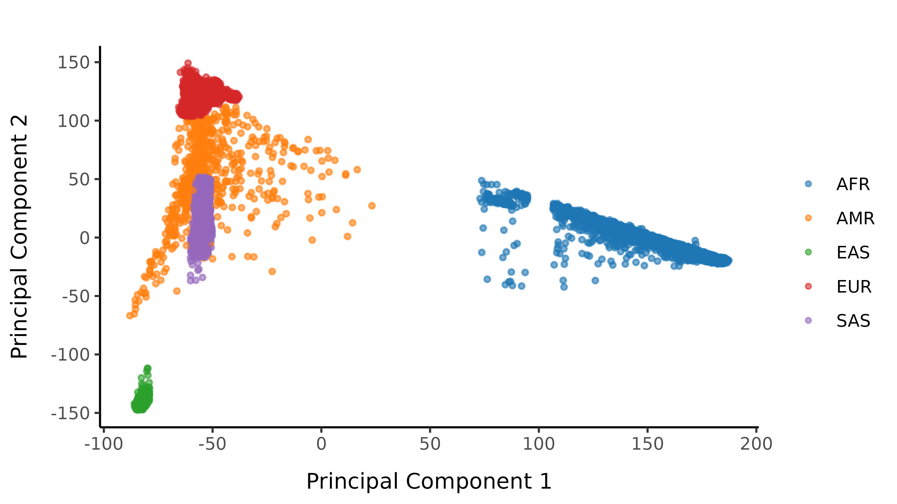
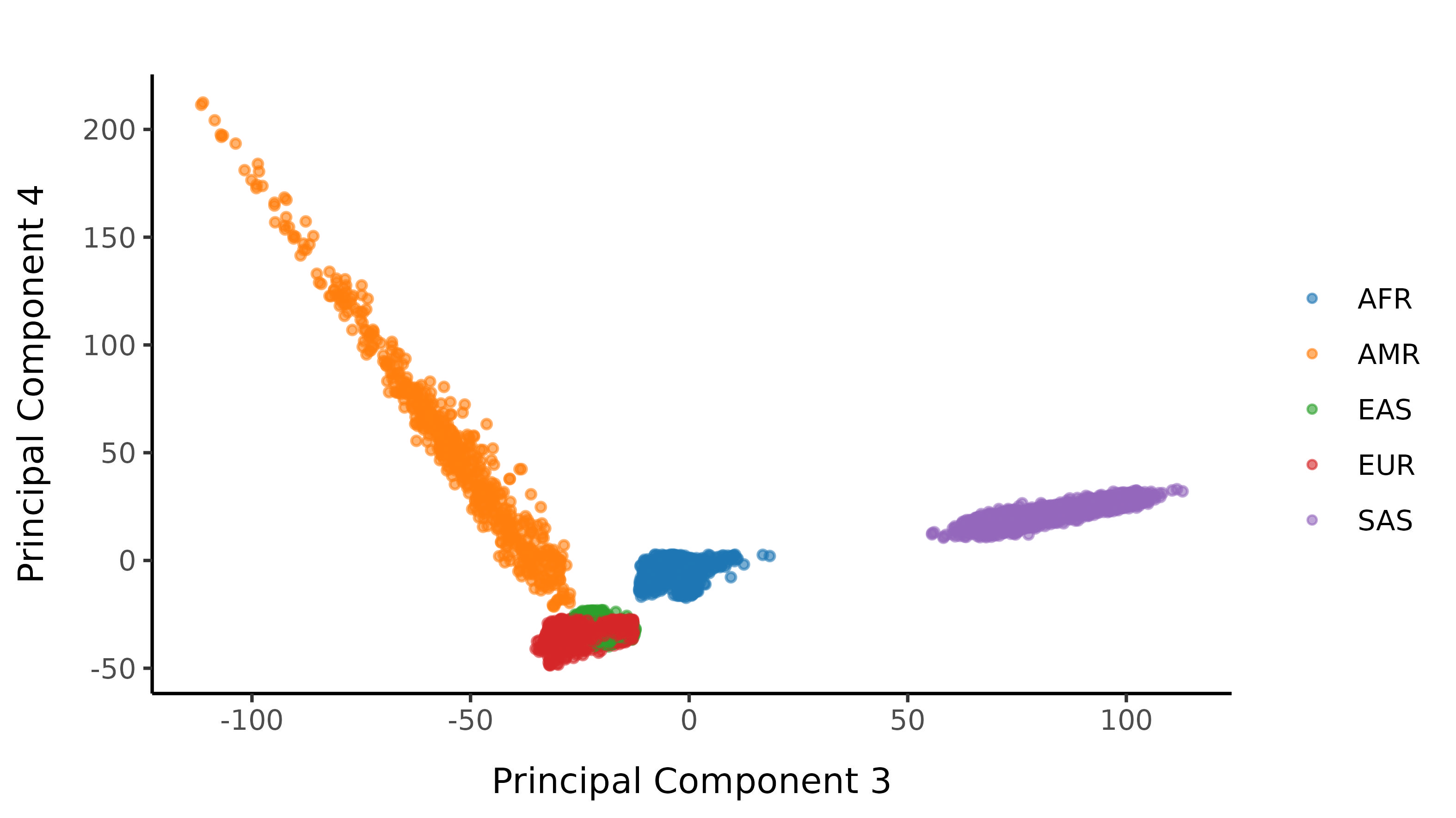
Subsequent filters are applied stratified by 1000G population labelling.
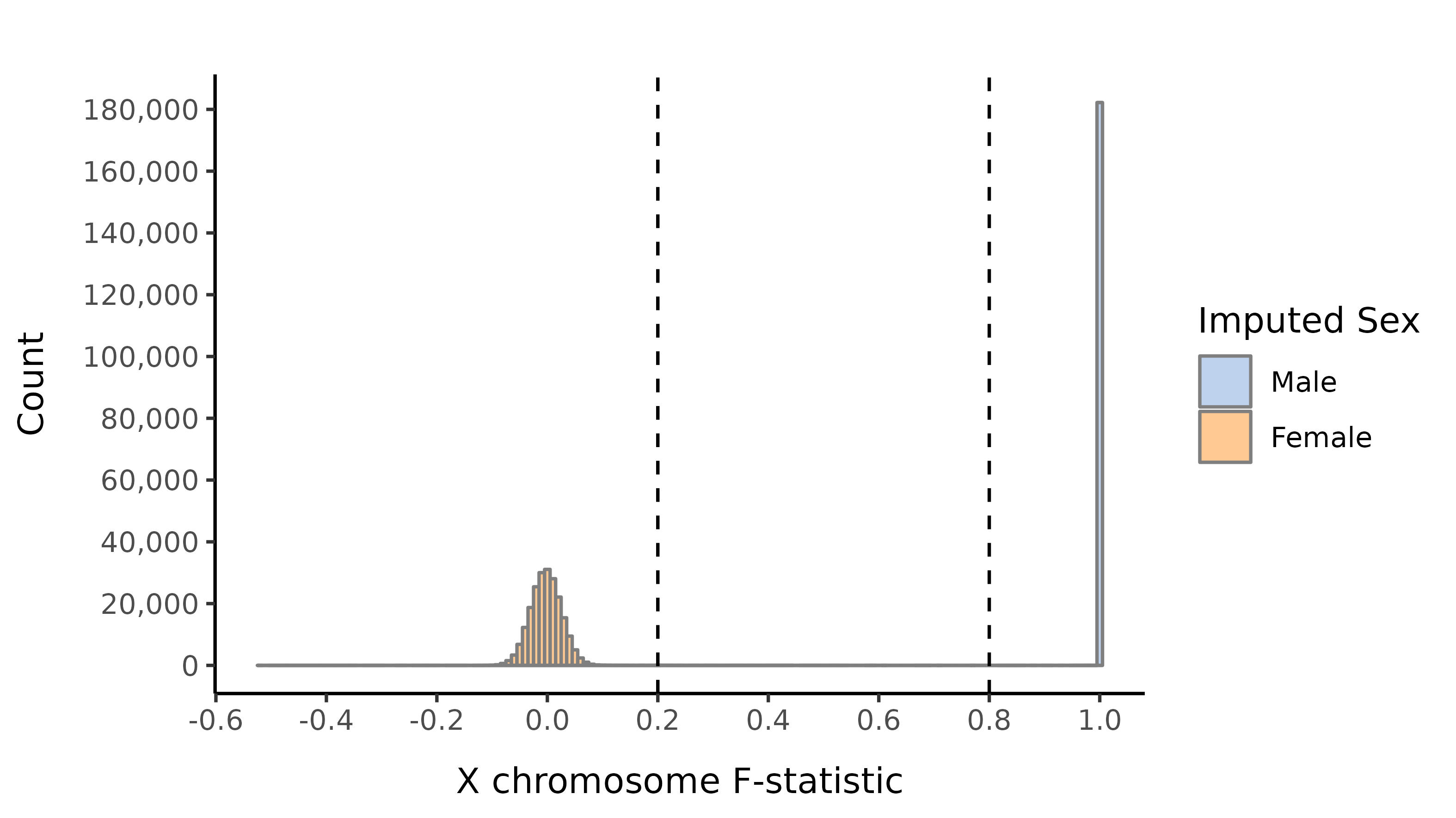
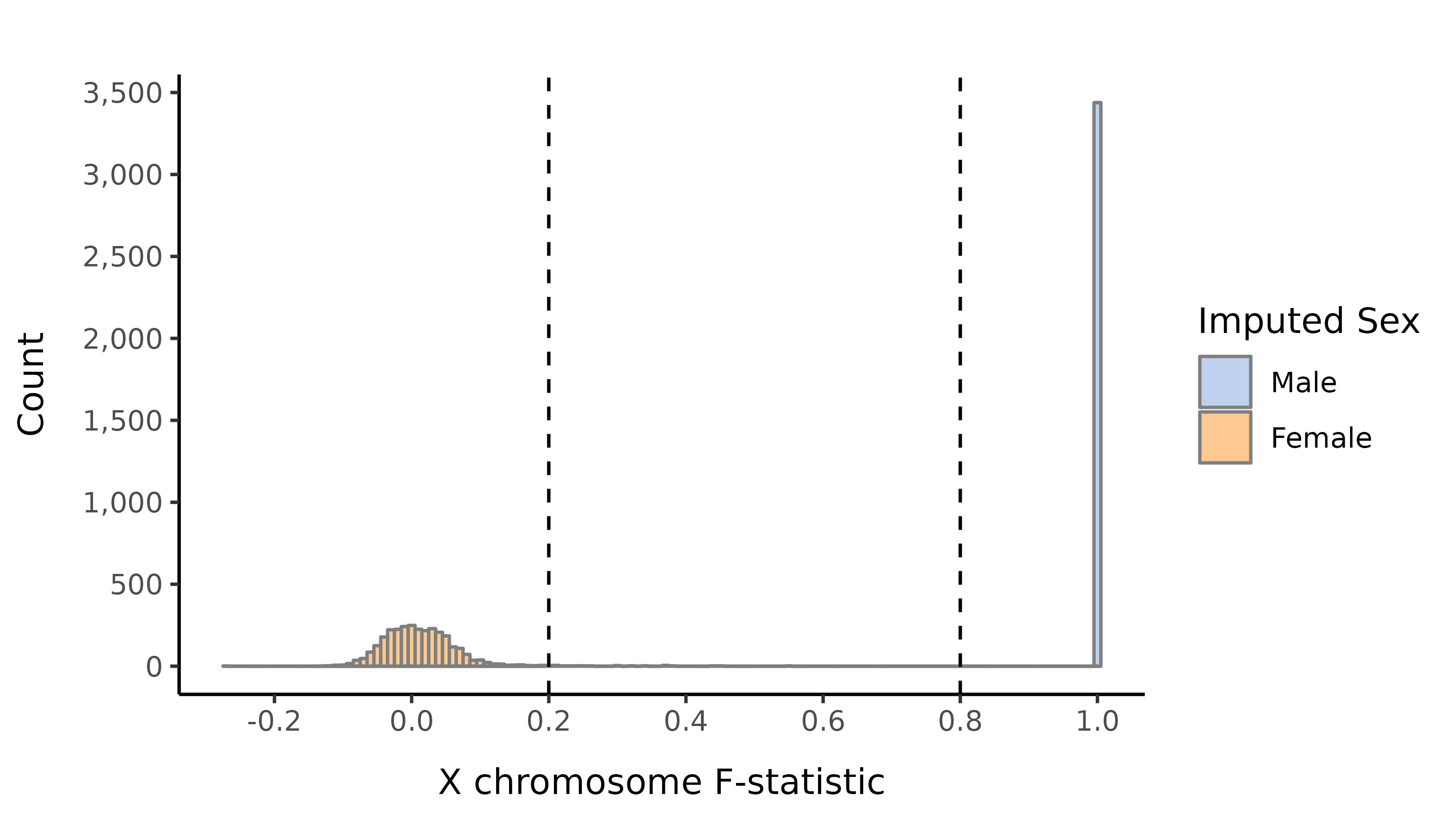
Sex imputation
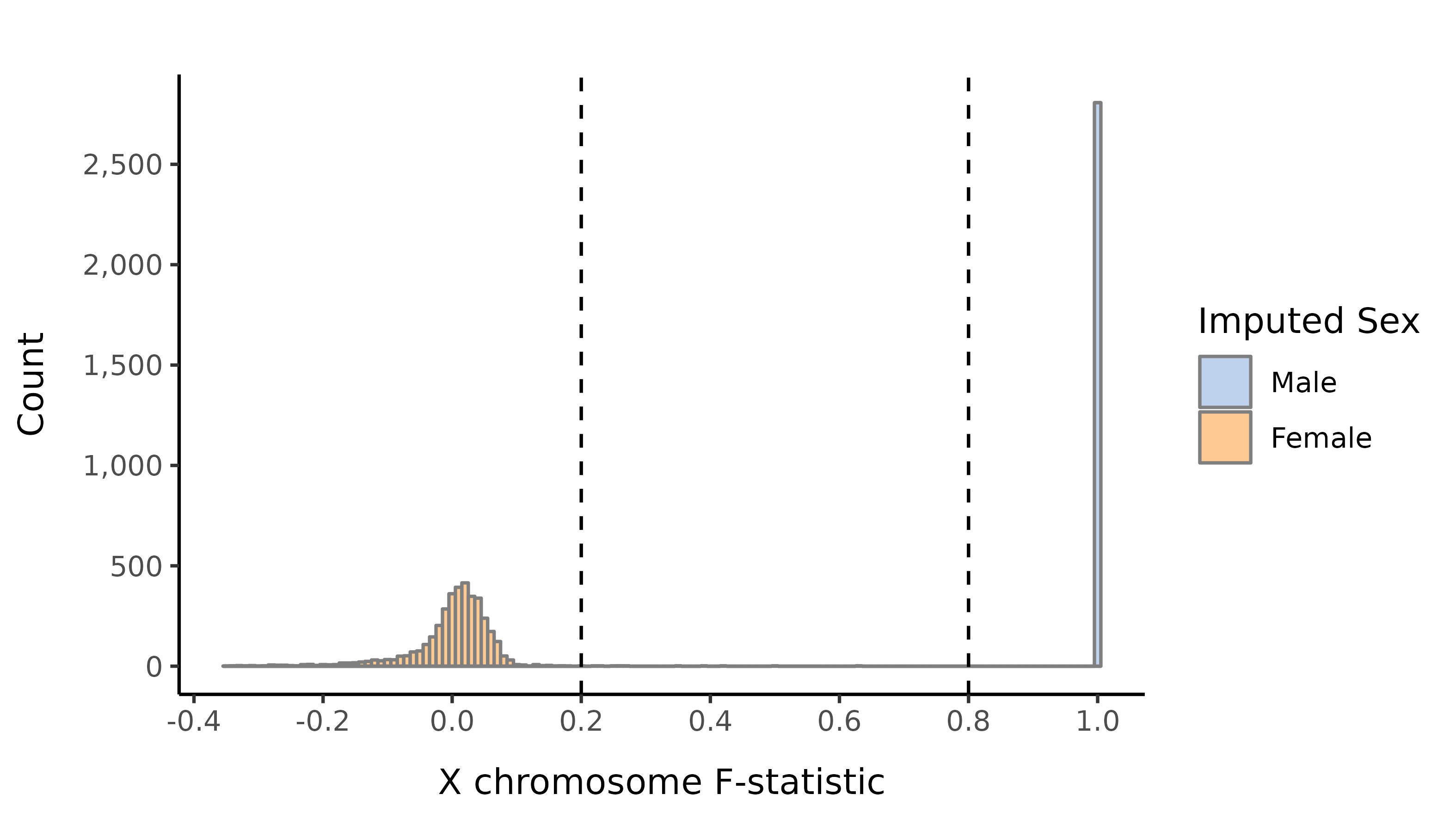
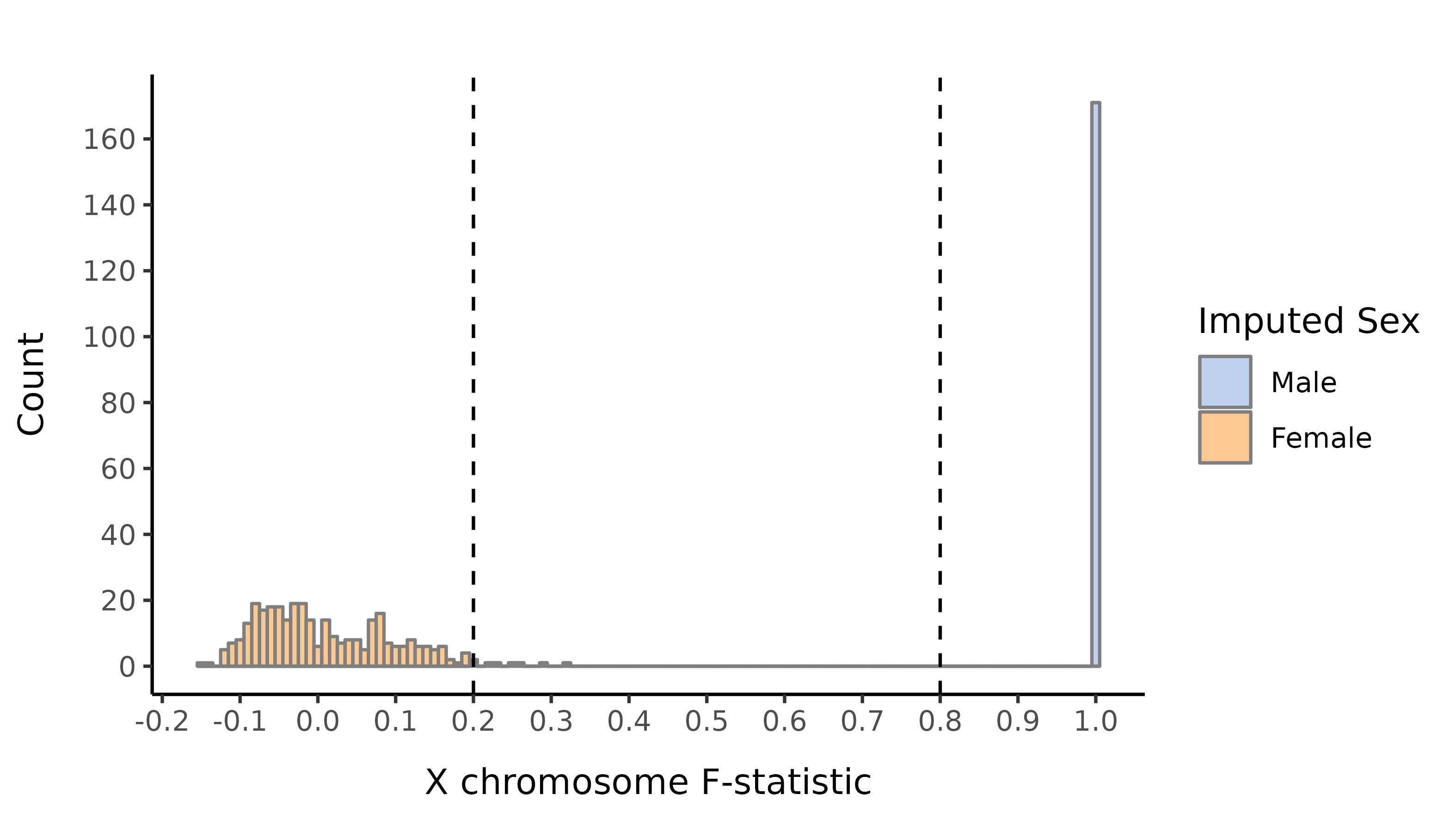
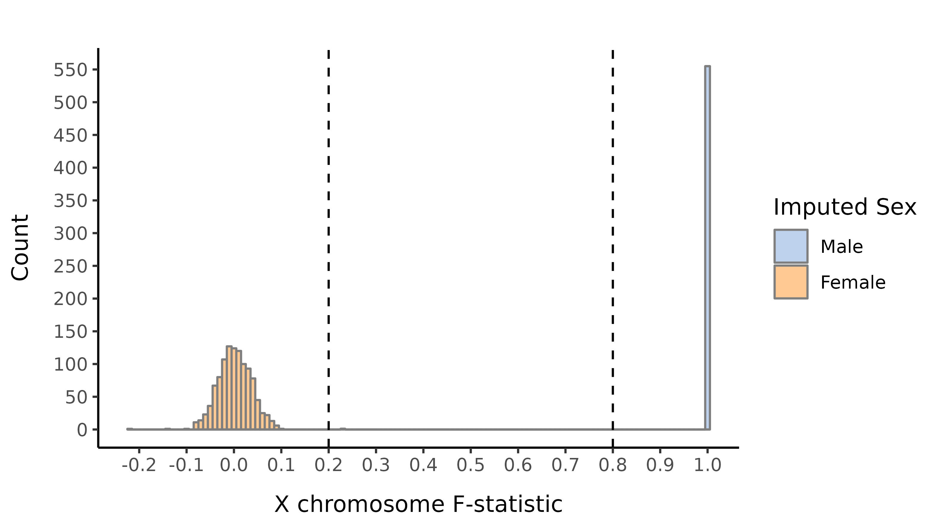
We impute the sexes of the individuals with this pruned set of variants on the X chromosome, and create list of samples with incorrect or unknown sex as defined by:
- Sex is unknown in the phenotype files
- F-statistic \(>\) 0.8 and the sex is female in the phenotype file
- F-statistic \(<\) 0.2 and the sex is male in the phenotype file
- F-statistic \(>\) 0.8 and number of calls on the Y is \(<\) 100.
- F-statistic lies in the interval (0.2, 0.8).
Here we show the distribution of the F-statistic, with the 0.2 and 0.8 thresholds defining our sex impututation shown as a dashed lines.
AFR
AMR
EAS
EUR
SAS
| Label | Before | Removed | After | % |
|---|---|---|---|---|
| AFR | 6,613 | 12 | 6,601 | 99.8 |
| AMR | 496 | 7 | 489 | 98.6 |
| EAS | 1,651 | 1 | 1,650 | 99.9 |
| EUR | 396,901 | 219 | 396,682 | 99.9 |
| SAS | 6,432 | 30 | 6,402 | 99.5 |
| Total | 412,508 | 269 | 412,239 | 99.9 |
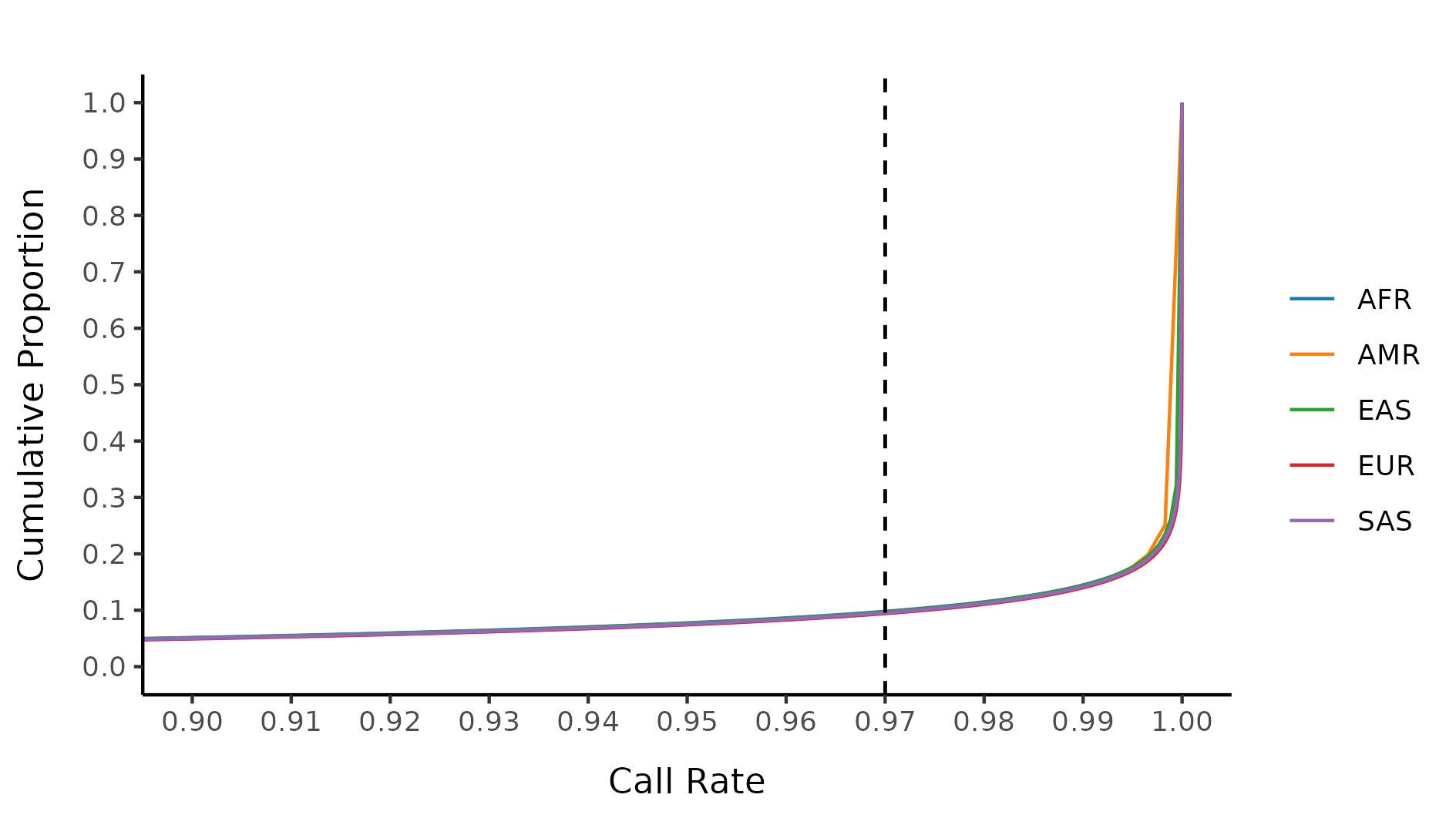
Final variant filtering
For our final variant filtering step, we first restrict to samples with strictly defined 1000G labellings, filter out samples with incorrectly defined sex or unknown sex, and run variant QC. Stratifying by 1000G labelling, we then evaluate a collection of variant metrics and remove variants that satisfy at least one of:
- Invariant site in cleaned sample subset
- Call rate \(<\) 0.97
- P-HWE \(<\) 10-6
The following plots shows the 0.97 threshold for call rate.
AFR
| Filter | Variants | % |
|---|---|---|
| Variants after initial filter | 18,992,636 | 100.0 |
| Invariant sites after sample filters | 16,364,165 | 86.2 |
| Overall variant call rate | 281,328 | 1.5 |
| Variants failing HWE filter | 6,614 | 0.0 |
| Variants after filters | 2,345,760 | 12.4 |
AMR
| Filter | Variants | % |
|---|---|---|
| Variants after initial filter | 18,992,636 | 100.0 |
| Invariant sites after sample filters | 18,336,374 | 96.5 |
| Overall variant call rate | 78,151 | 0.4 |
| Variants failing HWE filter | 1,100 | 0.0 |
| Variants after filters | 576,716 | 3.0 |
EAS
| Filter | Variants | % |
|---|---|---|
| Variants after initial filter | 18,992,636 | 100.0 |
| Invariant sites after sample filters | 18,001,198 | 94.8 |
| Overall variant call rate | 107,126 | 0.6 |
| Variants failing HWE filter | 2,391 | 0.0 |
| Variants after filters | 883,080 | 4.6 |
EUR
| Filter | Variants | % |
|---|---|---|
| Variants after initial filter | 18,992,636 | 100.0 |
| Invariant sites after sample filters | 3,216,967 | 16.9 |
| Overall variant call rate | 1,485,220 | 7.8 |
| Variants failing HWE filter | 23,574 | 0.1 |
| Variants after filters | 14,284,267 | 75.2 |
SAS
| Filter | Variants | % |
|---|---|---|
| Variants after initial filter | 18,992,636 | 100.0 |
| Invariant sites after sample filters | 16,671,965 | 87.8 |
| Overall variant call rate | 232,199 | 1.2 |
| Variants failing HWE filter | 4,939 | 0.0 |
| Variants after filters | 2,087,425 | 11.0 |
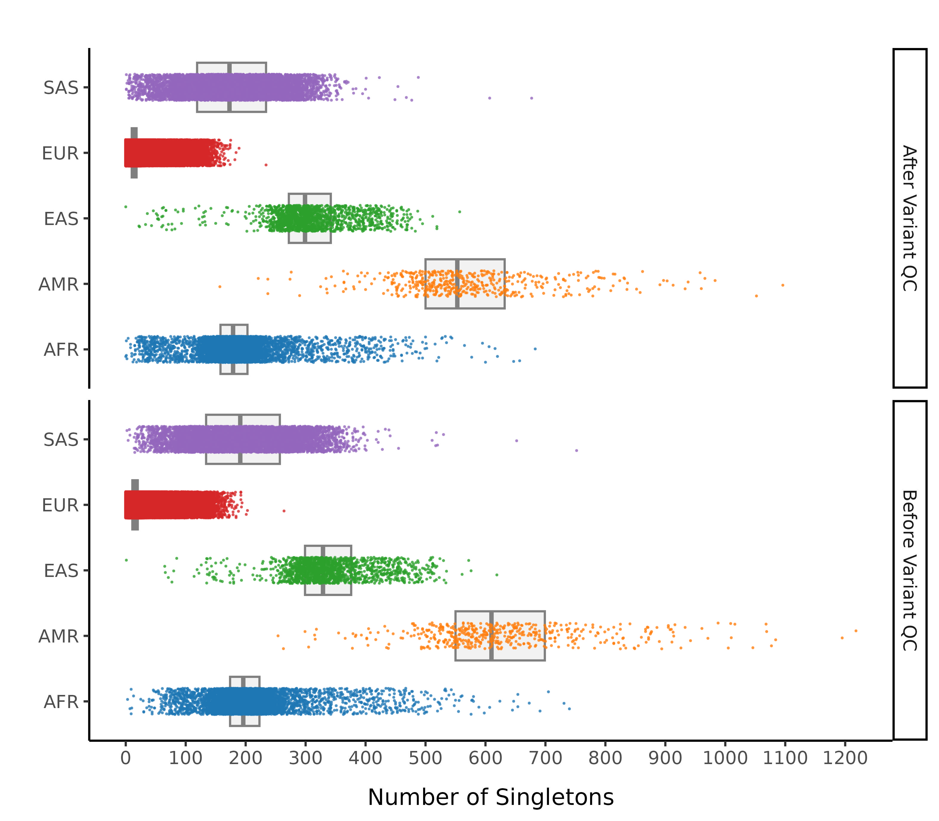
After these steps we plot the resulting changes in metrics across the samples in our data set. Each of this first set plots splits the data by 1000G label. The first collection of subplots in each figure shows the variant metrics before sample removal, with the lower collection of subplots showing the resultant change after our QC steps.
Number of Singletons
Ratio of Heterozygous to Homozygous Variants
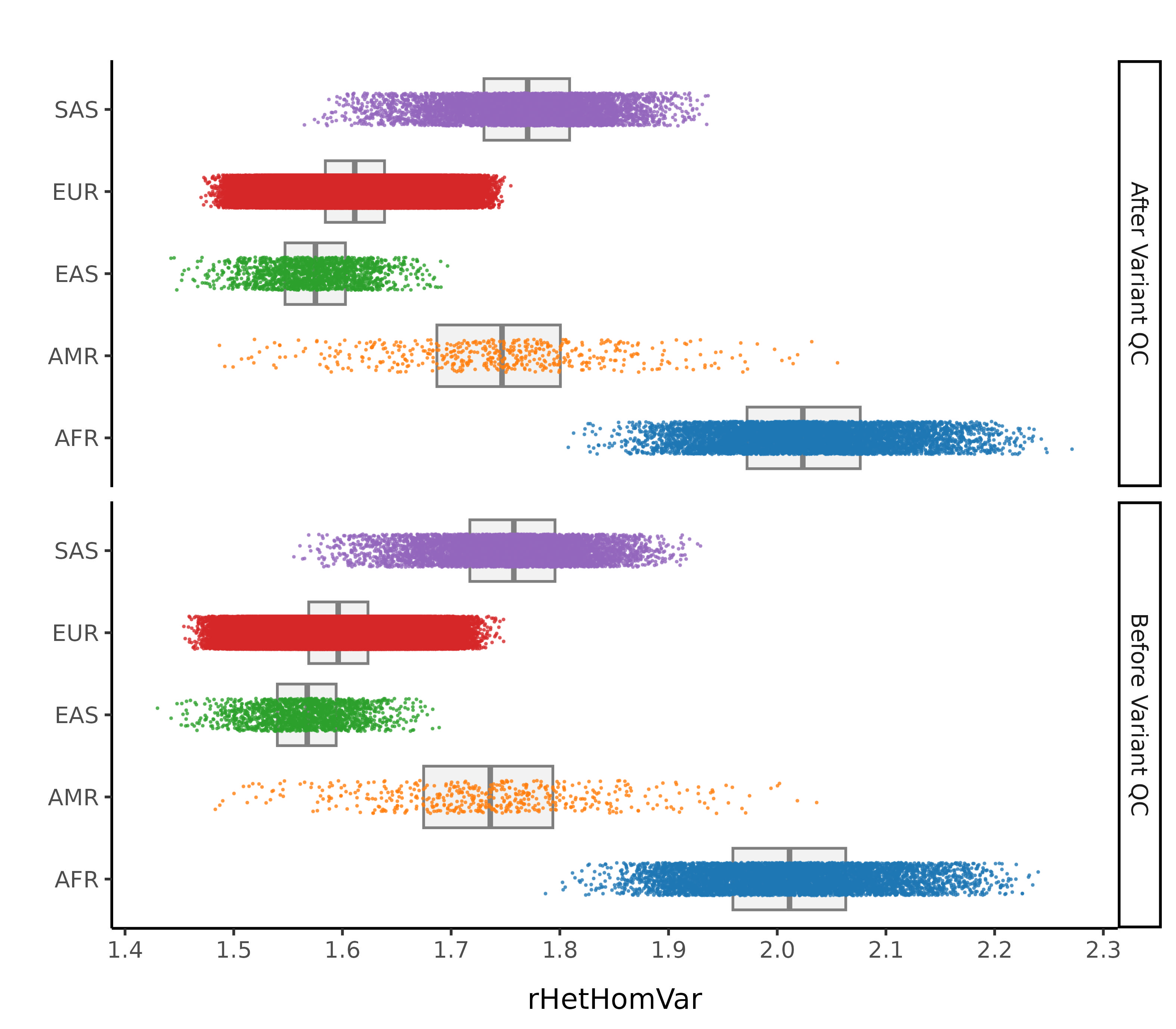
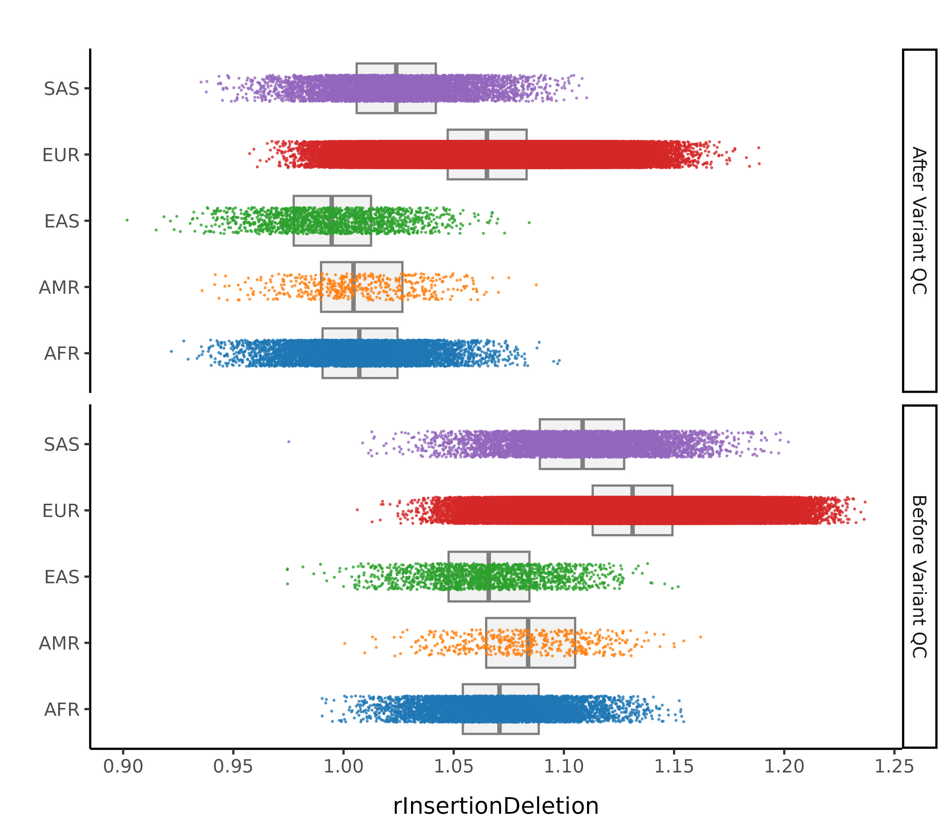
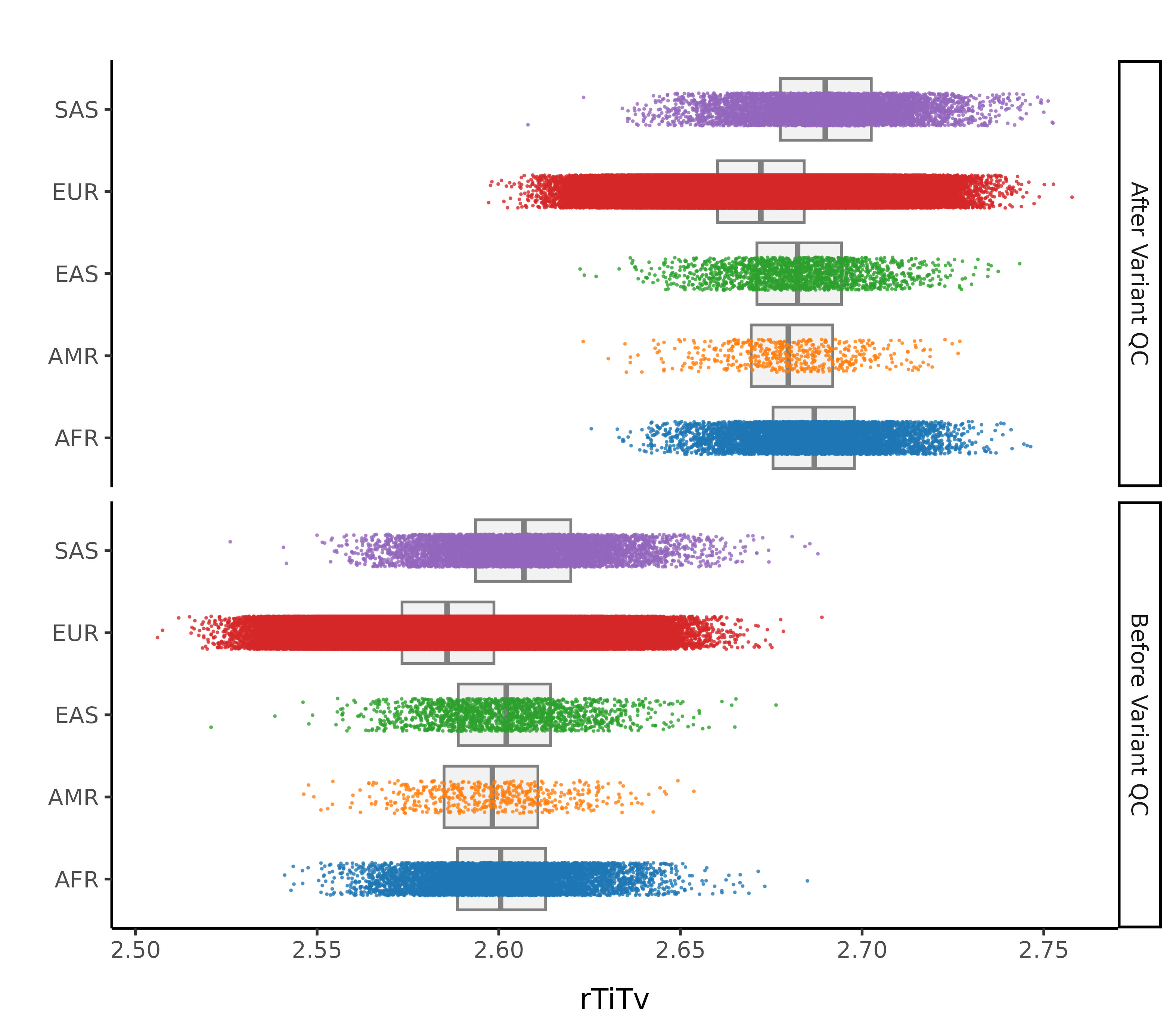
Final sample filtering
In this step we remove sample outliers after the variant cleaning in the previous step. Samples are removed if at least one of the following lies more than 4 standard deviations away from the mean (corresponding to a MAD threshold of 5.9304):
- Ratio of transitions to transversions
- Ratio of heterozygous to homozygous variant
- Ratio of insertions to deletions
| Filter | Samples | % |
|---|---|---|
| Samples after population filters | 6,601 | 100 |
| Within batch Ti/Tv ratio outside 5.9304 standard deviations | 0 | 0 |
| Within batch Het/HomVar ratio outside 5.9304 standard deviations | 0 | 0 |
| Within batch Insertion/Deletion ratio outside 5.9304 standard deviations | 0 | 0 |
| n singletons > 20 median absolute deviations | 0 | 0 |
| Samples after final sample filters | 6,601 | 100 |
AMR
| Filter | Samples | % |
|---|---|---|
| Samples after population filters | 489 | 100 |
| Within batch Ti/Tv ratio outside 5.9304 standard deviations | 0 | 0 |
| Within batch Het/HomVar ratio outside 5.9304 standard deviations | 0 | 0 |
| Within batch Insertion/Deletion ratio outside 5.9304 standard deviations | 0 | 0 |
| n singletons > 20 median absolute deviations | 0 | 0 |
| Samples after final sample filters | 489 | 100 |
EAS
| Filter | Samples | % |
|---|---|---|
| Samples after population filters | 1,650 | 100 |
| Within batch Ti/Tv ratio outside 5.9304 standard deviations | 0 | 0 |
| Within batch Het/HomVar ratio outside 5.9304 standard deviations | 0 | 0 |
| Within batch Insertion/Deletion ratio outside 5.9304 standard deviations | 0 | 0 |
| n singletons > 20 median absolute deviations | 0 | 0 |
| Samples after final sample filters | 1,650 | 100 |
EUR
| Filter | Samples | % |
|---|---|---|
| Samples after population filters | 396,682 | 100.0 |
| Within batch Ti/Tv ratio outside 5.9304 standard deviations | 0 | 0.0 |
| Within batch Het/HomVar ratio outside 5.9304 standard deviations | 0 | 0.0 |
| Within batch Insertion/Deletion ratio outside 5.9304 standard deviations | 0 | 0.0 |
| n singletons > 20 median absolute deviations | 277 | 0.1 |
| Samples after final sample filters | 396,405 | 99.9 |
SAS
| Filter | Samples | % |
|---|---|---|
| Samples after population filters | 6,402 | 100 |
| Within batch Ti/Tv ratio outside 5.9304 standard deviations | 0 | 0 |
| Within batch Het/HomVar ratio outside 5.9304 standard deviations | 0 | 0 |
| Within batch Insertion/Deletion ratio outside 5.9304 standard deviations | 0 | 0 |
| n singletons > 20 median absolute deviations | 0 | 0 |
| Samples after final sample filters | 6,402 | 100 |
Final Sample Counts
After all of this data cleaning, we save the resultant data for downstream analyses.
The composition of the samples according to 1000G labelling was as follows:
| Label | Count |
|---|---|
| AFR | 6,601 |
| AMR | 489 |
| EAS | 1,650 |
| EUR | 396,405 |
| SAS | 6,402 |
| Total | 411,547 |